Equity Hedging vs. Tail Risk Hedging

Equity Hedging vs. Tail Risk Hedging

Equity protection solutions can be broadly divided into two categories: tail risk hedging (TRH) and equity downside hedging (EDH):

• TRH: Solutions aiming to generate large returns in the event of an equity market sell-off of more than 25%
• EDH: Solutions that aim to generate positive returns in falling equity markets with relatively limited losses in rising equity markets

The definitions themselves illustrate the main mechanism by which the two strategies impact investors’ portfolios: TRH aims to cut-off the left tail of return distributions while EDH aims to reduce potential losses and portfolio volatility. TRH programs are often benchmarked to highly convex put option strategies, e.g., 3M 25% OTM (3M25) puts ⁽¹⁾, while EDH programs would be more closely aligned to longer dated put options struck closer to the money, e.g. 1Y 10% OTM puts (1Y10) strategy⁽²⁾. While the choice between these two programs often depends on each investor’s specific circumstances, we believe the following variables are the most salient for investors’ decision making:

Analysis of Benchmark Returns

Traditionally investors think about options in terms of their notional exposures. For example, we would usually say that a 10% OTM put option would pay-off 15% if the market went down 25%. However, in the world of equity hedging investors tend to think in terms of pay-offs per dollar spent. Thus, we will focus our analysis on the modified version of the strategies, where at each rebalancing day an investor spends 1% of its equity account notional on buying options: 3-month options in case of 3M25strategy and 1-year options in case of 1Y10 options.

Even though shorter-dated 25% OTM options trade at elevated implied volatility, they are much cheaper than 10% OTM annual options in absolute terms. Thus, for the same amount of dollars, investors can buy a significantly larger notional amount of these options. For example, a 25% OTM option expiring in 90 days, with implied volatility of 35% would cost approximately 0.25% of the notional, which means that on a rebalancing date an investor can buy 4 aa options. A one-year, 10% OTM option with an implied volatility of 23% would trade at ~3.5% of the notional, which means that this strategy would own 1.14x options – a much lower leverage than that of the 3M25 strategy.

But how frequently should we expect these options to pay-off? The difference is quite dramatic. In the last 64 years, quarterly 25% OTM options would expire in the money less than 1% of the time, while 10% OTM options would settle in the money about 13% of the time. This difference in probabilities indicates that the two strategies require different type of evaluation.

The table below provides a summary of performance of the two strategies since 3/31/1999 as well as the unlevered version of returns for each strategy. (Unlevered returns mean that the strategies maintain puts exposure equal to 100% of the account).

The performance differences are further illustrated by considering annual returns presented in the chart below.

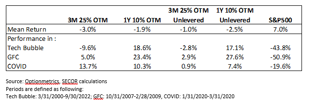
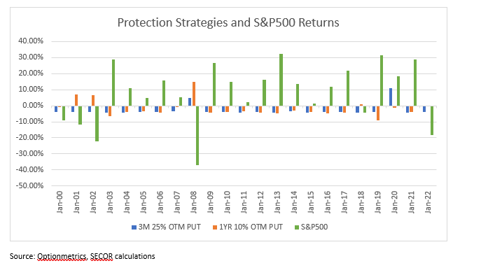
The table and the chart indicate that apart from the COVID sell-off, 1Y10 strategy provided a much stronger crisis performance than 3M 25% OTM. The differences were particularly stark during the technology bubble unwind, when a bear market lasted for a long time and 10% OTM options frequently settled in the money while 25% OTM 3-month options expired worthless.

The table also demonstrates that implementing the strategies with a constant-spent premium impacts performance differently depending on the type of equity sell-off: it helps when the sell-off starts from a very low level but hurts in the environment of GFC. It also helps when sell-offs are not large as the constant premium strategy does not buy as many options when they are expensive.

Evaluating Strategies

It’s particularly important to note that since options periodically settle in-the-money, the realised annual bleed for both strategies were lower than the 4% per year annual premium spent. Thus, investors should not equate an option premium with an expected cost of the program, it is much more accurate to evaluate the programs in terms of their expected return, which would depend on their benchmark and assumptions about manager alpha.

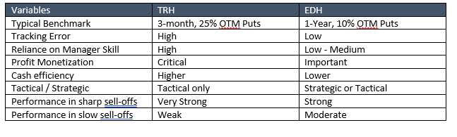
Given that 3M25 benchmark has a much higher bleed, why do some investors prefer this type of the program? The answer is three-fold: (i) it may provide higher convexity, (ii) TRH managers tend to monetise options before they expire, and (iii) betting on extreme outcomes usually allows managers to source protection somewhat cheaper than simply buying 25% OTM equity options.

Convexity profile is indeed more attractive for the 3M25strategy. Using the option, mentioned in the above example, which was priced at $0.25 at the time of the purchase, if equity markets went down 20% in one month after the purchase and implied volatility increased to 50%, the price of the option would increase to $5.4 – a 21x increase. The forementioned annual option would “only” increase in value 5.3x. Thus, when betting on extreme events 3M25 appears to be more attractive if the timing of this bet is extremely accurate.

Timing of monetisation and manager’ skills are much more important for the 3M25 program since without intervention, its bleed is double that of the 1Y10 program. Thus, TRH managers tend to have much higher tracking error to their benchmark than EDH managers. Furthermore, TRH managers aim to identify opportunities to create exposure to large equity market events by using exotic options, which may benefit from changing market correlations and events in fixed income or FX markets. This tends to reduce premium spent, but further increases tracking error.

Since EDH managers need to deliver smaller alpha for the program to break-even over the long-term, their need for tracking error budget tends to be lower. While they can use the same strategies as TRH managers, a set of simpler tools may also provide value. For example, they can substitute a portion of benchmark exposures with either other, relatively cheaper option structures, such as spreads, or even with linear strategies such as Trend. Given their lower tracking error, 1Y10 benchmark provides better guidance for long-term returns and, therefore, maybe easier to evaluate for a strategic allocation within institutional framework.

Conclusion

We believe that the two types of protection strategies discussed in this note – TRH and EDH – have their unique characteristics and their evaluation requires different approaches. Given TRH strategies’ higher reliance of managers alpha, these strategies are more likely to end up in an “alpha” or “special opportunities” bucket, while EDH strategies maybe better suited for strategic allocation since their benchmark and alpha requirements maybe better understood.

Strategy and Index definitions below:

• SPX 10% OTM Put is a portfolio of 10% out-of-the money (OTM) puts with 3, 6, 9 and 12-months maturities on S&P500 Index. At each quarterly option expiration, 1-year, 10% OTM put option is purchased with a notional exposure equal to 25% of the assumed notional.
• All purchases of options are done at the Asking price, at the end of the day.
• All options are held to maturity.
• Assumed account notional is constant over time.
• Quarterly Option Expiration is a third Friday of March, June, September, and December.
• Performance only includes profits or losses from holding options. Daily percentage return is calculated as the sum of all dollar profits and losses from all options held in the portfolio divided by the Assumed Account Notional.

Any questions regarding this document or the disclosures above should be directed to cco@secor-am.com.

(1) The 3M 25% OTM Put strategy assumes buying 3-month 25% OTM put option on S&P500 index, on the account notional amount, on the third Friday of March, June, September and December; the value of the account is assumed to be the same at each rebalancing.

(2) The 12M 10% OTM Put Strategy assumes buying a one-year, 10% OTM put option on S&P500 index, on 25% of the account notional amount, on the third Friday of March, June, September and December; the value of the account is assumed to be the same at each rebalancing.